Purpose of this webpage is to investigate the numbers we get with different measurements of colocalization, such as Pearson's correlation, simply how much overlap particles have, or other methods, of 2D images. For instance, is a spatial relationship of puncta really strong evidence of interactivity? A large part of this depends on the biological system. Vesicles or lysosomes may contain molecules that are there with the only relevance being that they are being degraded. Or maybe the molecules really have a functional interaction, even if by intermediaries. Or maybe they don't have direct interactions but are within the resolution of the system. And within the noise of the imaging system. Unless explicitly stated otherwise, the puncta below really are or are simulated to represent clusters of many molecules. Think of the resolution of the system as each voxel being 0.13 X 0.13 X 0.5 um and one optical section through a 3D volume. A specific protein in cell nucleii was imaged.
I first encountered this problem presented in a seminar in the mid- to late-1990s and this paper from the Fay and Singer group then in Worcester, MA explains, "The image from one probe was translated with respect to the other in three dimensions to compare colocalization with random alignments." They cited a paper from a year earlier that decribed the method in more detail in its Figure 3. I accepted that simple translation (including rotation or mirror imaging) would work as a surrogate for randomizing in irregular biological specimens and subsequently used this.
So let's play and test this.
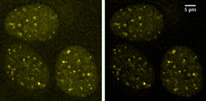
On the left, the "original" image and on the right a contrast enhanced version. This is yellow because there is a red channel and a green channel. We are pretending each channel is a different protein for the sake of providing a sample with 100% colocalization.
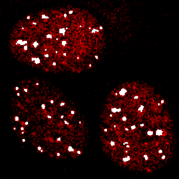
An initial step has to be segmenting the features of interest, in this case the bright puncta in the nucleii. Problem seen in this simple threshold is that red puncta are missed; increasing decreasing the threshold to grab them also pulls in too much background.
Therefore, we applied a local contrast enhancement with radius of 25 pixels to try to make the puncta have more equivalent intensities which would facilitate simple thresholding.
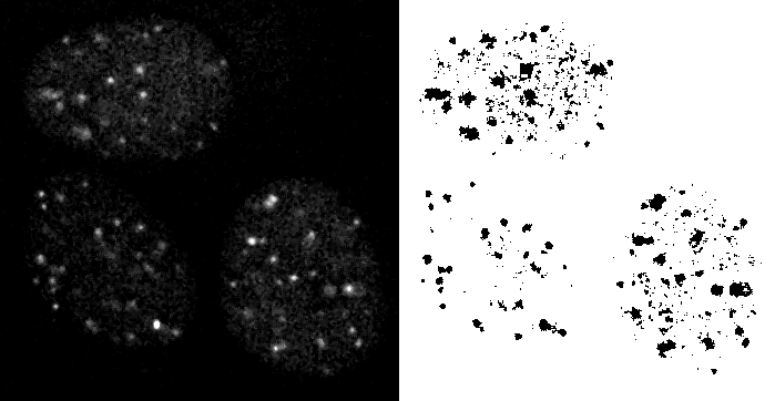
Because the result had a lot of single pixel noise, an erosion was applied to remove them and then a dilation applied to bring the larger objects back to approximately their original size.
The result still may not be perfect, but it's a lot closer to what I think I see by eye and what we're going to use for the rest of the tests.
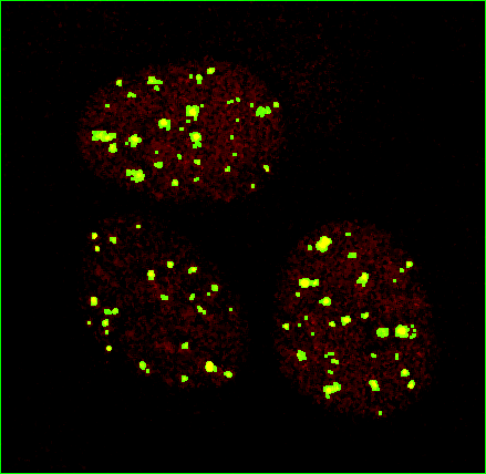
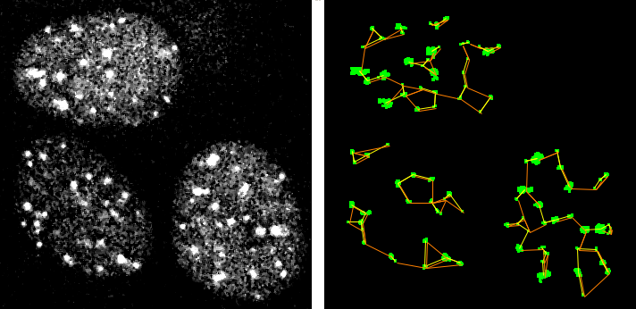
A tangent: clustering. The following image has the problem of only being from a single optical section of a 3D cell nucleus, but this analysis or segmenting could be extended to 3D. For a description of what this represents, please see clustering webpage and the measurements here were generated with this macro.
The segmentation above would be useful for looking at relationships between particles and the masks could also pass the raw data to apply Pearson's correlation. But let's take a step back and look at Pearson's applied to the raw data.
What is r=? What happens when shifted? Used macros at http://microscopynotes.com/imagej/colocalizationspotssimulation/index.html and Pearson's through time webpage repackaged as colocalization_and_labelling_macros_used.txt.
Question: How does shifting the data by a few pixels change the Pearson's correlation, a.k.a. "r ="?
![]()
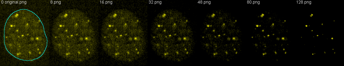
The get the below results for r =, the images were converted to 8 bits and thresholded (a constant subtracted) at increasing values to reduce background and priviledge bright structures. All three cells were measured independently and results averaged. Pictured here are the example thresholds for one of the cells and how it was segmented for the measurements.
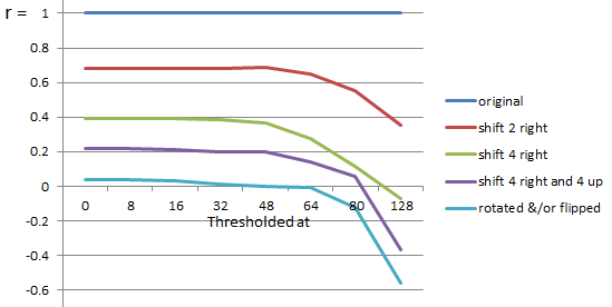
| Thesholded at | 0 | 8 | 16 | 32 | 48 | 64 | 80 | 128 |
| original | 1.00 | 1.00 | 1.00 | 1.00 | 1.00 | 1.00 | 1.00 | 1.00 |
| shift 2 right | 0.68 | 0.68 | 0.68 | 0.68 | 0.69 | 0.65 | 0.55 | 0.36 |
| shift 4 right | 0.39 | 0.39 | 0.39 | 0.39 | 0.37 | 0.28 | 0.12 | -0.07 |
| shift 4 right and 4 up | 0.22 | 0.22 | 0.21 | 0.20 | 0.20 | 0.14 | 0.06 | -0.37 |
| rotated &/or flipped | 0.04 | 0.04 | 0.03 | 0.01 | 0.00 | -0.01 | -0.12 | -0.56 |
More analysis and better macros for automation.
This does not address the question whether the results are different than when the images are a random distribution rather than linear shifts, although I would argue that a linear shift of irregular distributions would yeild the same result as random, but this simulation is for a different day.
Another way people like to show these data is with linear intensity plot profiles.
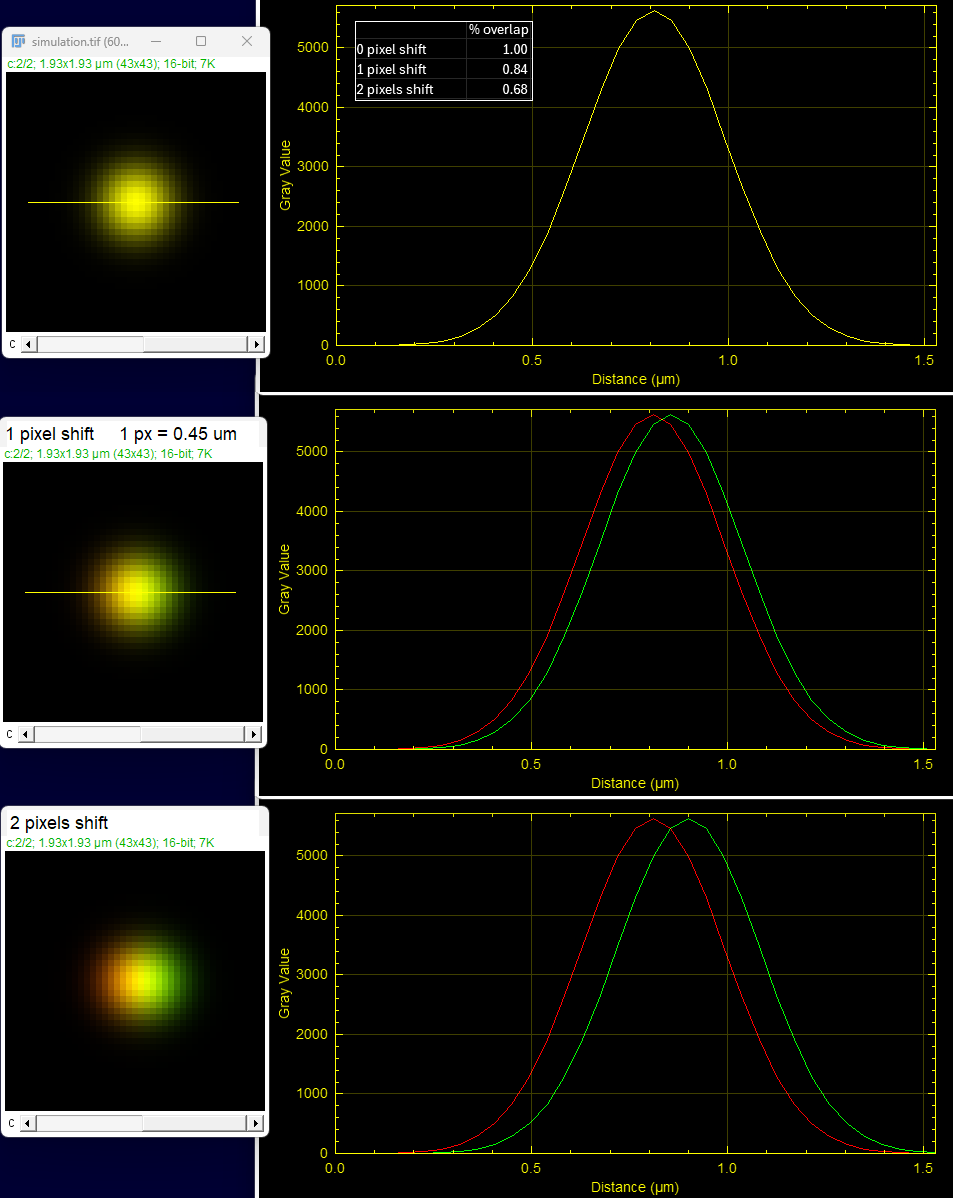
These plot profiles were created using the macro for multicolor plot profiles in MC_macros.ijm (as of July 2025).
When the peaks of the curves are at the same location, there is colocalization.
In this example, for a group of fluorescent molecules smaller than the resolution of the microscope, only the top image is colocalized. The other two examples show the discrete aggregation of molecules in each channel abutting or near each other.
As to statement in Fay et al., "full dynamic range needs to be considered...", don't underestimate how one bright pixel is enough to alter r=. Show this with an example.
What about thresholded % overlap? Calculate per particle. This is really the question from seminar Dec 2016 as they dismissed Pearson's.
There was also a question about shape change and biological relevance, but this is not addressed here; it's a different question. Same with size & intensity change.
And looks like there's a lot of literature on this (and I bet a lot of redundant software but not shareable because very tailored to each lab's imaging modalities formats).
last updated 20161212_1153 mcammer@gmail.com