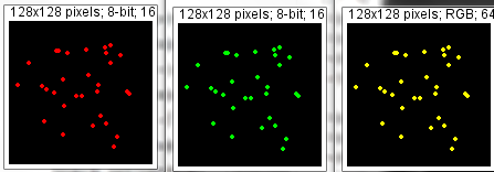
the red and green dots all merge to make yellow. They are 100% colocalized. Pearson's correlation r = 1.
This is an example of why maximum projection (or other projection method) 2D images from Z stacks of optical sections cannot be used for most analysis, in this particular case, colocalization. (Also for spatial distance, not addressed here.)
Projections superimpose images from XY locations in a stack of images into a single image, thus the uniqueness of the Z location is lost.
Based on this image
the red and green dots all merge to make yellow. They are 100% colocalized. Pearson's correlation r = 1.
However, this is wrong because the image is a maximum pixel projection of a Z series. The dots came from a Z series where most of them were not colocalized. They were in the same XY locations, but in different Z locations.
 |
 |
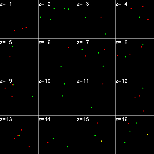
When analyzed in their original spatial locations within a volume sampled by thin slices, most of the objects are shown to not colocalize. Only in z = 9, 15, 16 is there any colocalization and only in z = 15, 16 is the colocalization the same spots. (Simulation made with CZ_simulation_v100.txt)
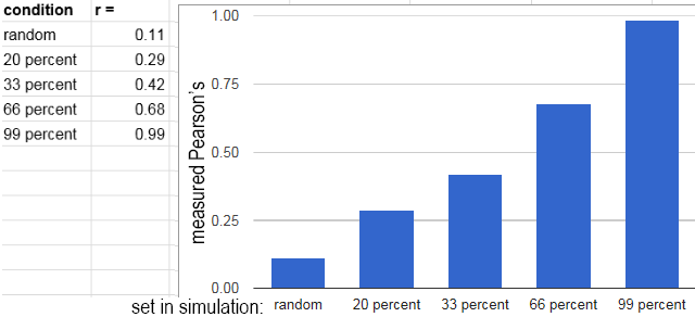
This simulation can be made a bit less blunt by adding known amounts of colocalization. (CZ_simulation_v100_with_defined_percentage.txt)
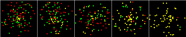
From left to right, the percentages of colocalization were preset as
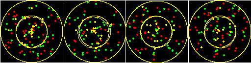
random, 20%, 33%, 66%, 99%. 900 spots distributed over 16 images was used. The images below are single examples. The chart is an average of 12 of the 16 images from each condition.
The simulation could also be modified to change colocalization based on geometry. The simulation was designed to keep the spots in a circle to have a modicum of resemblance to a cell stuck to a coverslip. Putting an if statement in to look at the random part of the amplitude is a simple way to make the center of the cell and band around the outside have different colocalization coefficients. is < 0.5, make the chances of colocalization some percentage greater with an additional random() call and < or > 0 to 1.
This would make the center of the cell have a greater colocalization coefficient than the exterior band.
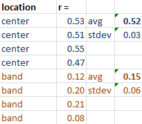
In this example the inner circle with radius 0.66 of the total radius has 50% of the spots colocalized and the outer band is random. (CZ_simulation_v100_with_defined_percentage_geometry.txt)
Something else to consider is that the spots are randomly distributed along the radii. The means that near the center, the spots are going to have a higher concentration. With higher numbers of spots, these jumble together. This may have consequences for misinterpreting light microscope images taken at the limit of resolution or with saturated intensities.
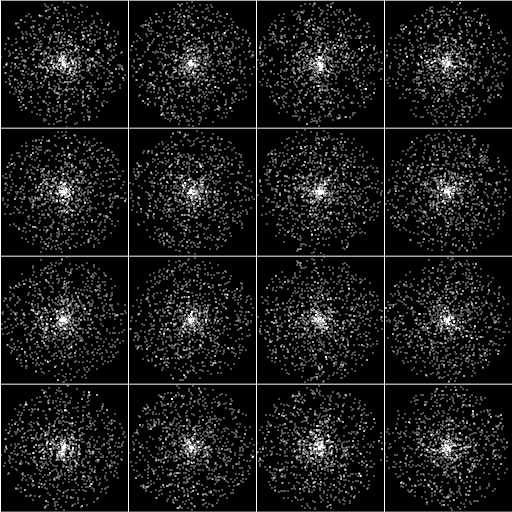
The simulation above is 900 spots of each red and green distributed over 16 cells where the spots remain mostly discrete.
The image immediately below is 30 times the spots distributed over 16 cells.
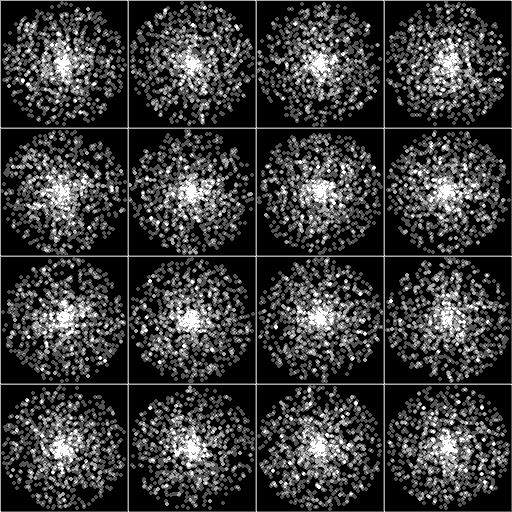
Even when the spots are smaller, the center is higher concentration. However, the distribution from center to periphery is statistically equal along radii.
Macro used for Pearson's: colocalization_for_RGB_v105.txt
last updated 20150909_1338 mcammer@gmail.com