ImageJ notes
If you want to do pixel-by-pixel colocalization analysis on timelapse images, it is essential that the images be taken simultaneously.
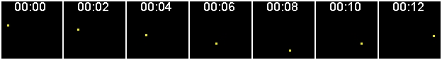
This series of images simulates a red and a green particle collected at precisely the same time. Two examples of simultaneous imaging are confocal where two detectors collect the colors at the same time and a beamsplitter that projects the two different colors onto different sides of the same camera that takes frame snaps that are not progressive.
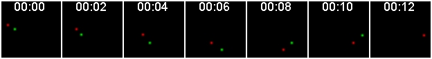
This series of images simulates sequential imaging. This is typically done where one color is collected, then a filter turns, then the next color is collected. Obviously, pixel-by-pixel colocalization will return a zero correlation answer.
Need to make sure there is no spillover from one channel to the other. Controls of imaging condition need to be performed before full experimental data collected. Some computational cross subtraction may be valid based on controls.
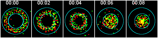
Similarly, ensemble particles imaged simultaneously
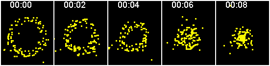
and sequentially
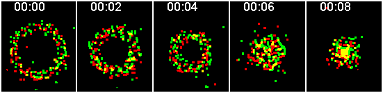 .
.
If the particles are dense enough, radial profile plots may track the movement of an ensemble. In the below graphs, the top graph is time 00:00 going down to the bottom which is 00:08. From left to right is spatial, from the cell center to the periphery. And the Y axis is intensity. Note that the intensity scale changes and at 00:08, there is a plateau in the graph at the center of the cell; this is saturation.
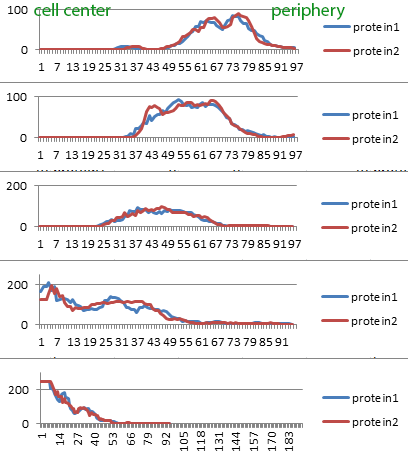
These radial profile plots were created using the macro "Radial Profile Plot multiple cells from overlays [q]" with a separate run for each timepoint.
Also, colocalization can be measured on a region-by-region basis but the definition of colocalization is, again, molecules in same region but no conclusions can be drawn about interacting. This is a much simpler way of showing the same phenomena.
Here one region is a band at the outside of the cell and the other region is the central portion of the cell. It is clear that both proteins translocate from the annulus to the center at the same rate. They migrate together regardless whether they interact. (Yes, the intensities are normalized.)
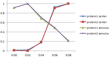
The annulus vs. central portion may be done directly by measuring on the images or by integrating over segments along the radial profile plot.
More Here and More Here and Through Z or Time
What is the yellow pixel? Sort of an answer here.
above content last updated 20141013_1427
All data above with my macros. Fiji has a built in colocalization module that returns the same values for r Analyze > Colocalize Threshold
20180529
Costes et al Automated and Quantitative Measurement of Protein-Protein Colocalization of Live Cells, Biophysical Journal, June 2004 is a well written paper for simple explanation of colocalization. However, despite its arguments to the contrary, it remains a method for measuring above a threshold. Whether this threshold is background, low concencentration of relevant protein per pixel, or relevant are distinctions that would have to be argued on a case by case basis.
As for methods, from green to red, in our experience, requires no chromatic aberration corrections. Depending on the lens, however, blue and far red probes need correction. CFP and YFP typically do require correction by shifting the focal plane. Whether PSF is really relevant depends on the sample type, for example, small isolated puncta vs broad volumes. For red and green labeled mitochondria with a high N.A. planapochromat & single pinhole, in our opinion, not an issue.
comments, questions, suggestions: Michael.Cammer@med.nyu.edu