Scans were collected at 1024 x 1024 pixels, speed 400 Hz, Zoom factor 2.0 to produce 90.19 nm pixels with a 63X N.A. 1.4 oil lens. The sample is cultured mammalian cells fixed and labeled with AF488-phalloidin by Molecular Probes.
This web page discusses balancing the gain and laser intensity combined with averaging or accumulation to collect high quality confocal images with the Leica Stellaris microscope. Most of this discussion may be applied to other Leica confocals with HyD detectors.
Perhaps the biggest problem we find with confocal images is that they are saturated. This masks fine resolution and prevents quantification of images. A misconception is that brighter images ae better images. The goal is to have the best signal. Signal is related to dynamic range and noise, not what you find pleasing on the screen as brightness.
There are a few ways to make the image brighter.
The biggest problem we have with compromised image quality is saturation and we want to make sure all users learn how to avoid this.
The HyD detectors on the Leica confocals are photon counting devices and image quality purists argue that they should always be used in photon counting mode. However, we have found that this adds layers of complication for training users for most practical use of the confocal for biological imaging, especially if they are already familiar with earlier or other models of laser scanning confocals. Also, photon counting collected images often have a grainy quality which people do not like. Therefore, we train based on a compromise mode of imaging.
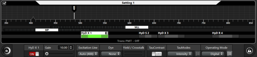
When using HyD detectors, there is a base gain setting. For instance, on our Stellaris, detectors X1, X3, and R4 have a minimum gain setting of 10. Detector S2 has a minimum setting of 2.5.
We recommend that detectors X1, X3, and R4 be set from 10 to 20.
Detector S2 be set from 2.5 to 10.
They should not be set higher than 25 or 10 ever; this would make images noisy without adding any real information. (see 1 above).
Therefore, to get more signal out of a sample, you need to turn up the laser. However, turning up the laser too high will result in pileup of photons and will not be linear. There are two examples as you read below.
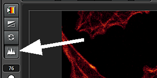
All images shown below are using the glow over LUT (look up table) and screen snapped from the LASX software diaplay.
Scans were collected at 1024 x 1024 pixels, speed 400 Hz, Zoom factor 2.0 to produce 90.19 nm pixels with a 63X N.A. 1.4 oil lens. The sample is cultured mammalian cells fixed and labeled with AF488-phalloidin by Molecular Probes.
First, a discussion of the histogram.
| The intensity histogram shows the number of pixels at each intensity value. The X axis is the values of the intensities running fomr 0 to 255 for 8 bit images and the Y axis is the frequency of each. |
 |
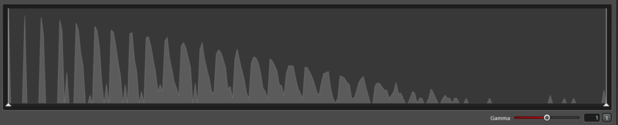
If the histogram has discrete peaks, then the gain is set too high. This adds no signal to the image and risks saturating the image.
Again, no matter how much
you think saturated images are pretty, they throw away signal. Do not collect data with saturated pixels.
(If you intentionally want individual peaks, then switch to photon counting mode.)
Histogram showing gain set too high resulting in discrete peaks:
Let's just call this a bad image.
Gain 147; Laser 1.8%
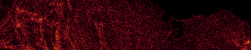
This can be corrected by dropping the gain and digitally adjusting the contrast.
Note that the laser setting is the same in these two images.
Gain 20; Laser 1.8%
For this detector (HyD X) with a minimum gain of 10, we recommend the gain set between 10 and 20. The histogram is smooth and the intensity range wide enough for precision intensity measurements. Increasing the gain will not add to the precision.
Increasing the laser a little may add to the dynamic range, but it rapidly leads to pile up of photons which makes the response non-linear and unacceptable for intensity quantification.
The histogram does not decay to the right and bumps up against saturation. (There is a second demonstration of this below where gain is 10 and the laser is 77%.)
This image is unacceptable for two reasons: 1.) laser set too high and 2.) saturated pixels.
Laser 78; photon counting mode.
Therefore, once you see signal, do not crank up the laser to see more.
[Add quantification data here with ground truth provided by low laser 16bit photon counting accumulation 16.]
A few examples of good and bad settings and how to adjust gamma to see weak signal in the same samples that have strong signal.
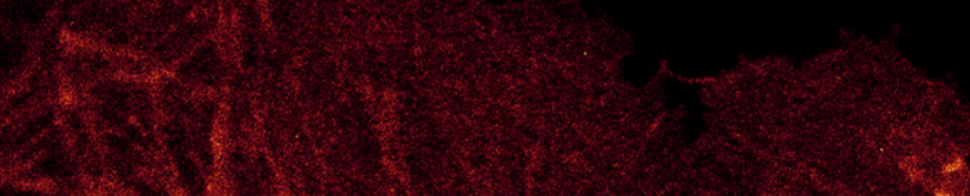
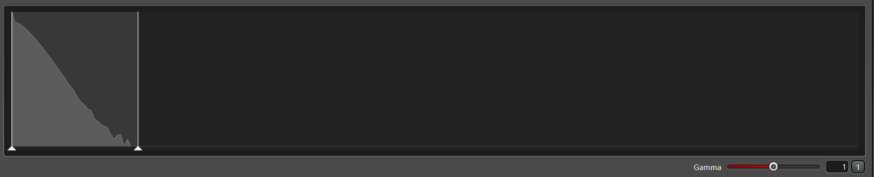
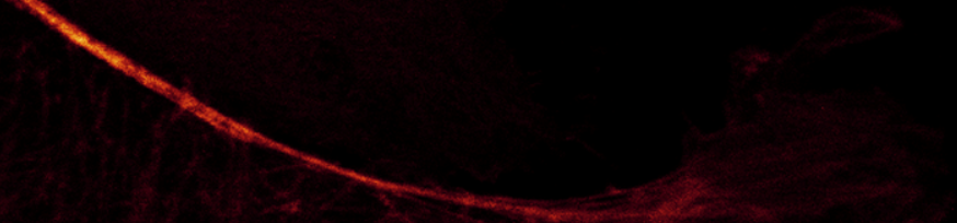
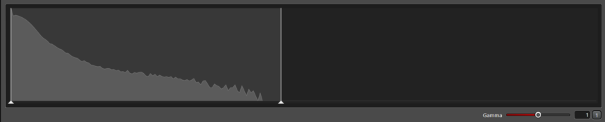
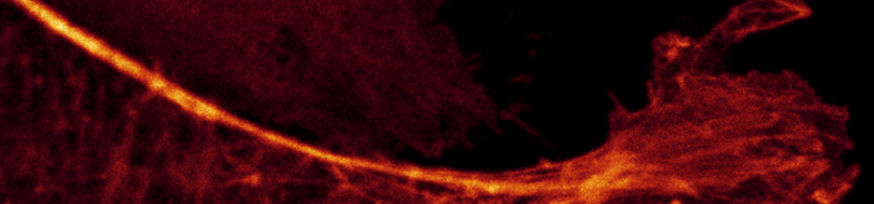
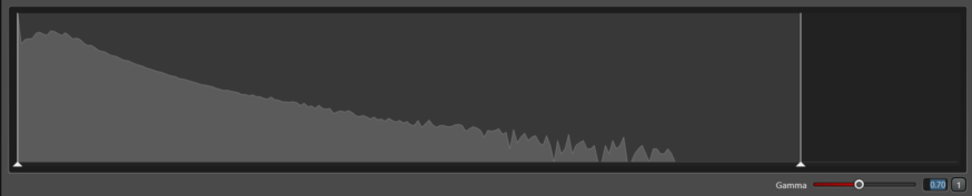
This image has a good dynamic range from dark to light and low noise for a single scan.
You do not see the information in the darks, but it is really there. It is revealed by adjusting the display contrast (next image).
Gain 10 (minimum); Laser 2%
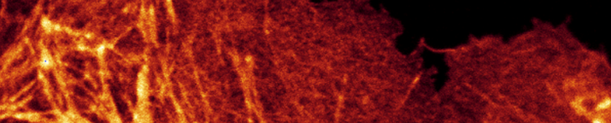
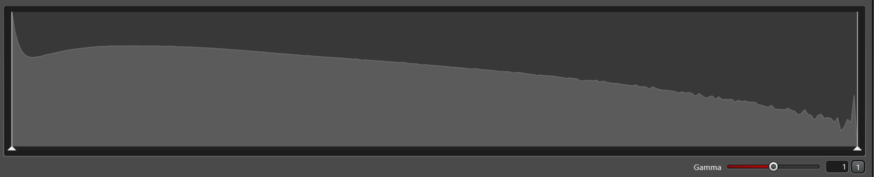
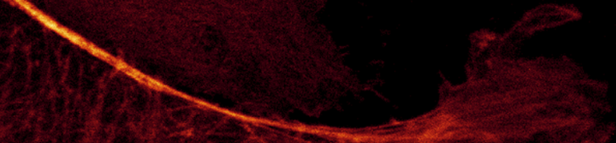
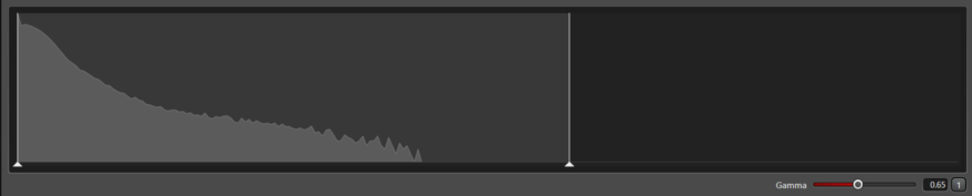
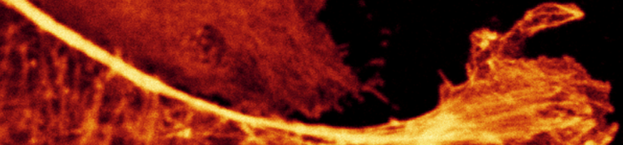
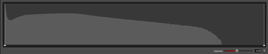
The only difference bewteen the this image, which clearly shows the low concentration f-actin in the dark areas without saturating the f-actin bundles in the bright areas, is the contrast setting in the display. In the lower right of the histogram, note that the gamma is set to 0.65. This increases the brightness and contrast of the lower intensity pixels without saturating the brighter ones. This does not change raw data; it only changes the display of the data.
A typical "common sense" rationale for saturating one area of an image, for instance the cell body of a microglia or soma of a neuron, is, "Because I need to see the fine structures." Blasting the center of the cell isn't going to produce signal out at the processes. If the signal is there, it can be revealed by adjusting the gamma.
The images above and this image are examples of a good histogram.
The histogram in this image shows pixels that are brighter
because the laser intensity was set to 10% whereas the images above it was set to 2%.
Gain 11 (close to minimum); Laser 10%
This image shows a pileup of intensities (right side of the histogram). Setting the laser high in an attempt to make the image brighter resulted in a non-linear pileup of photons. This image should not be used for quantification because the dark areas do not have a linear relationship of number of molecules to the bright areas.
Note that so far, all images have only used 50% to 70% of the available dynamic range; there was no need to force the counts to fill the full 256 possible values in the range.
Gain 10; laser 77%
Conclusions:
The biggest misconceptions are 1.) that the gain setting provides more signal and 2.) that images need to be bright to the extent of saturation to see dim signal. Both these "common sense" notions need to be rejected. These misconceptions have been our biggest problem with training people how to collect high quality images which are both aesthetically pleasing and can be used for quantification.
A typical "common sense" rationale for saturating one area of an image, for instance the cell body of a microglia or soma of a neuron, is, "Because I need to see the fine structures." Blasting the center of the cell isn't going to magically produce signal out at the processes. There are things to try such as:
Turn the gain down and the laser up.
Adjust the focus (processes maybe in different focus planes and require a Z series with projection to see as a continuous structure).
Average for less noise.
Non-linear contrast adjustment for displaying the image (gamma).
16 bits instead of standard 8 bits.
Accumulation if there is time to acquire more photons (a.k.a. more signal).
Use a different lens.