Normal confocal integration detection vs photon counting.
I had always accepted that normal laser scanning confocal imaging with PMTs (photomultiplier tubes) was quantitative except for issues such as bleaching, pumping too much laser into the samples, overstaining, or other extremes. First I did this in practice, in 1991 working with Dr Richard Hays at Einstein College of Medicine looking at f-actin on the brush border of kidney proximal tubules compared to basolateral actin and told it could be quantitative by using an internal control [https://www.physiology.org/doi/pdf/10.1152/ajpcell.1992.262.3.C672]. [Later Nick Franki did the prep and I made the confocal micrograph in a different paper's Fig 2a.] Then in 1992 reading the first edition of James pawley's confocal bible. I found that in the BioRad MRC600, the instrument we had at the time, adjusting the ND filters for laser illumination yielded expected intensity changes as measured by the PMTs. The confocal became the go-to instrument for localized photometry, in particular for f-actin localization in the Condeelis lab. We were writing custom macros for NIH Image running on a Qudra 950 and 840 AV to measure protein concentration in specific cell compartments. It wasn't until 1995 that we got our first Photometrics cooled CCD camera with a KAF1400 chip for wider dynanic range quantitative widefield imaging. Regardless, there never was a question that if we stayed in the linear range of confocal settings, the results wer quantifiable linearly. The first ratio fluorescence talk that I remember was ast NYSEM or or other seminar in NYC from someone at Columbia, I think Dunn, and which I think was later published in this paper, where the confocal was used to look at pH very localized in (what they then called) endosomes. I don't know what they had to discuss with reviewers, but this work required confocal response as linear.
Why my rambling now? Circa 2013 I found that some confocal users were insistent on using photon counting mode of the confocal, a type of imaging no one I knew found necessary.
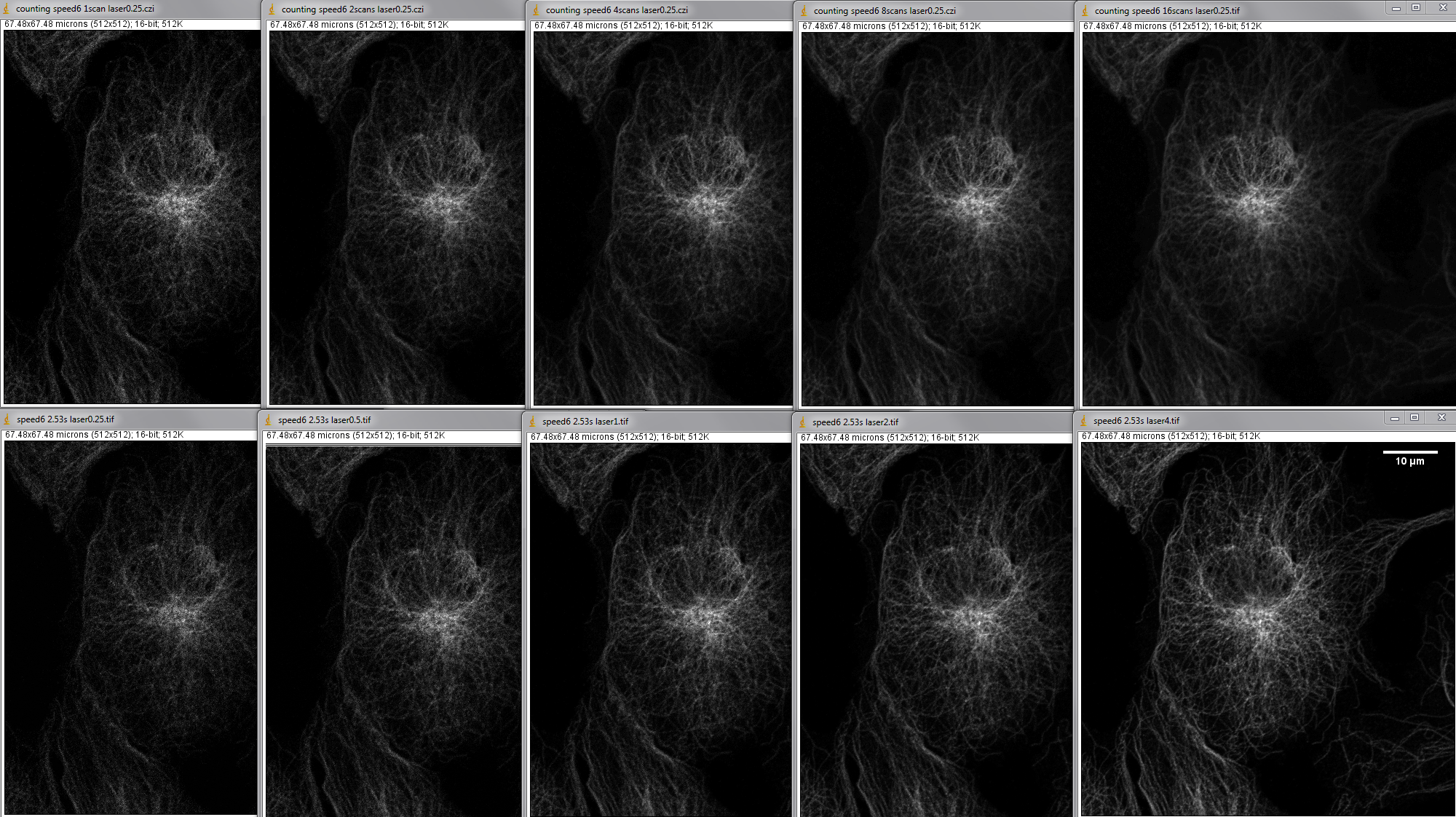
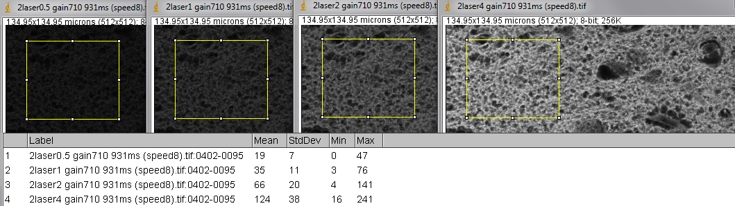
This image is normal confocal mode with laser power changed by 2X for each condition; see title bar at op of each image.
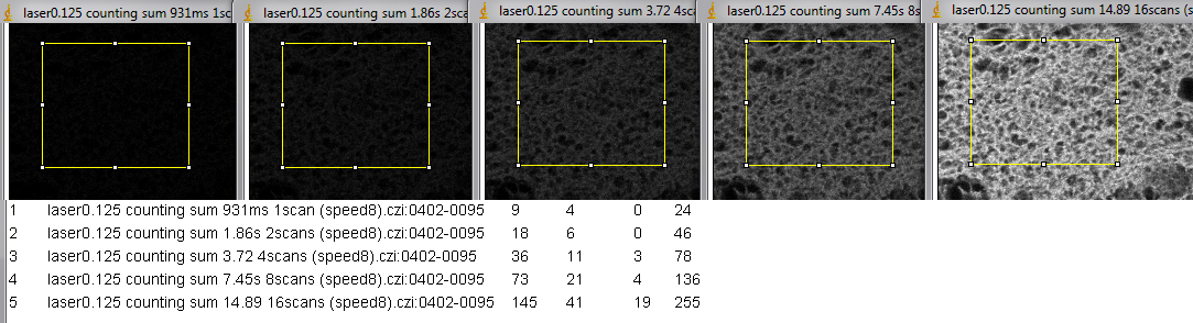
And now photon counting, which requires laser power below 0.5 as used in images above.
First column is mean intensity and second column is standard deviation.
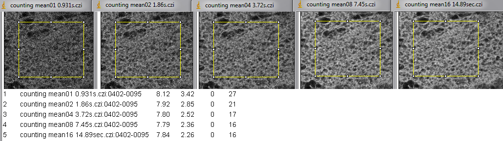
The figure below is the same area with images collected by two different methods.
Top row is photon counting with averaging set. The contrast for all images in the top row is the same. Each full field took 2.53 seconds per scan to image. The title bar says how many scans were averaged to collect the image.
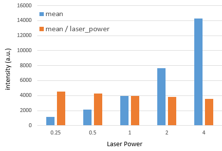
The bottom row is contrast stretched linearly min to max. Each image is a single scane at 2.53 second. The laser settings varied from 0.25 to 4 on the slider in the Zen software. Laser power measurments done a few days earlier showed that each halving/doubling of the number correlates directly with laser power.